Technical Visualization: The RAG System Architecture
Try our Open Source Assets for RAG Systems
AI RAG Chunkenizer
Document chunking for RAG pipelines. Process PDF, Word, Excel — 100% in browser. No data leaves your device.
Part I: The Fundamental Problem
Large language models possess remarkable capabilities but suffer from a critical architectural constraint: the context window. This window represents the maximum number of tokens (discrete units of text typically representing approximately four characters or three-quarters of an English word) that a model can process in a single inference call.
Even as context windows have expanded into the millions of tokens, enterprise reality renders them insufficient. A mid-sized organization might maintain 500,000 documents across contracts, technical specifications, internal communications, research papers, and operational records. A single legal discovery request might involve 2 million documents. Financial institutions routinely manage document repositories exceeding one petabyte. Converting these figures to tokens produces numbers that dwarf any context window: a petabyte of text documents translates to roughly 250 trillion tokens.
Beyond sheer volume, stuffing massive context windows creates practical problems. Inference costs scale with token count. Latency increases. Most critically, LLM attention mechanisms degrade with context length, models struggle to maintain focus across extremely long contexts, a phenomenon researchers call “lost in the middle” where information in the center of long contexts receives less attention than information at the beginning or end.
Retrieval-Augmented Generation addresses these constraints by decoupling knowledge storage from knowledge processing. Rather than forcing all information through the context window, RAG systems maintain external knowledge bases and retrieve only the specific information relevant to each query. The LLM receives a focused, manageable context containing precisely the passages needed to answer the user’s question.
Part II: System Architecture Overview
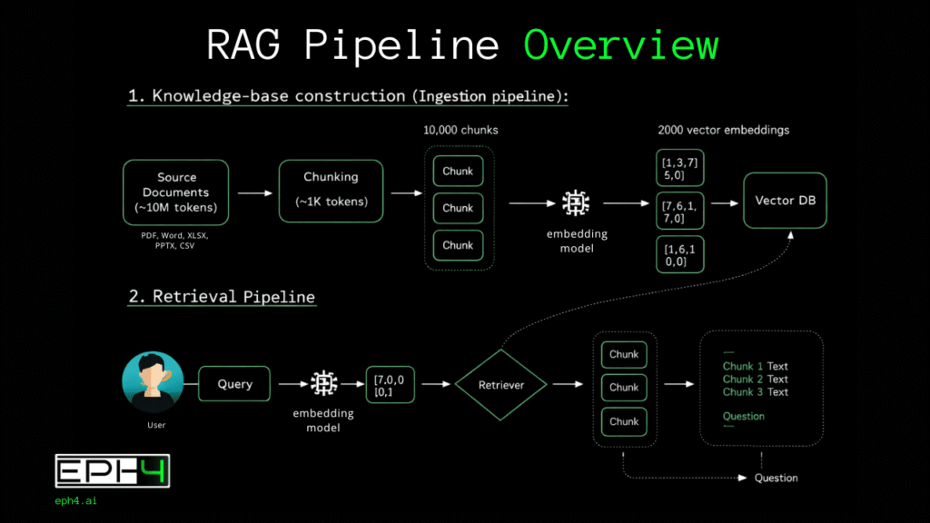
A production RAG system comprises two distinct pipelines operating asynchronously.
The injection pipeline (also called the indexing pipeline) processes source documents into a searchable format. This pipeline runs offline during initial system setup and periodically thereafter as new documents enter the corpus. Its output is a populated vector database containing mathematical representations of document content.
The retrieval pipeline (also called the query pipeline) handles real-time user interactions. When a user submits a query, this pipeline searches the vector database, retrieves relevant content, and orchestrates LLM response generation. Latency requirements are strict; users expect responses within seconds.
Understanding both pipelines in technical depth is essential for building systems that actually work.
Part III: The Injection Pipeline
Stage 1: Document Ingestion and Preprocessing
Raw documents arrive in heterogeneous formats: PDF, DOCX, PPTX, HTML, Markdown, plain text, scanned images requiring OCR, emails with attachments, spreadsheets containing textual data. The ingestion layer must normalize this diversity into clean, structured text.
PDF extraction presents particular challenges. PDFs are presentation formats, not semantic formats, they specify where characters appear on a page, not what those characters mean. Tables become scrambled text. Multi-column layouts interleave incorrectly. Headers and footers repeat on every page. Figures contain text that extraction tools miss or misplace. Production systems require specialized PDF parsers: libraries like PyMuPDF (fitz), pdfplumber, or commercial solutions like Amazon Textract or Azure Document Intelligence that apply machine learning to reconstruct document structure.
Metadata preservation matters significantly. Document titles, authors, creation dates, section headings, and source URLs provide crucial context during retrieval. A chunk stating “revenue increased 15%” means nothing without knowing which company, which quarter, which document. Injection pipelines must extract and associate metadata with each chunk.
Text cleaning removes noise that degrades embedding quality: excessive whitespace, special characters, encoding artifacts, boilerplate headers/footers, page numbers, and irrelevant formatting markers. However, aggressive cleaning risks removing meaningful content—code snippets, technical notation, structured data. Cleaning strategies must be tuned to document types.
Stage 2: Chunking Strategies
Chunking: dividing documents into retrievable units is where RAG systems succeed or fail. Poor chunking cascades through the entire system: embeddings capture wrong semantic boundaries, similarity search returns irrelevant results, and LLM responses hallucinate or miss critical information.
Fixed-Size Chunking
The simplest approach divides text into chunks of predetermined token count, typically 256 to 1,024 tokens. Implementation is straightforward: tokenize the document, split at regular intervals, optionally add overlap between consecutive chunks to preserve context across boundaries.
Document: [Token1, Token2, ... Token10000]
Chunk size: 512 tokens
Overlap: 50 tokens

Chunk 1: Tokens 1-512
Chunk 2: Tokens 463-974
Chunk 3: Tokens 925-1436
...
Overlap prevents information loss when important passages span chunk boundaries. Without overlap, a sentence beginning at token 510 and ending at token 520 would be split across chunks, potentially rendering both fragments semantically incomplete.
Advantages: Predictable chunk sizes simplify embedding model input management and retrieval token budgeting. Implementation requires minimal document understanding.
Disadvantages: Arbitrary boundaries ignore semantic structure. A chunk might begin mid-sentence, split a paragraph discussing a single concept, or combine the conclusion of one topic with the introduction of another. These semantically incoherent chunks produce embeddings that fail to capture meaningful content.
Sentence-Based Chunking
This approach respects grammatical boundaries by splitting only at sentence endpoints. Sentences are grouped until reaching a target chunk size.
Sentence boundary detection requires more than splitting on periods, abbreviations such as (Dr., Inc., U.S.), decimal numbers (3.14), and ellipses (…) create false positives. Production implementations use NLP libraries with trained sentence tokenizers: spaCy, NLTK’s Punkt tokenizer, or regex patterns tuned to specific document types.
# Conceptual implementation
sentences = sentence_tokenize(document)
chunks = []
current_chunk = []
current_length = 0

for sentence in sentences:
    sentence_length = count_tokens(sentence)
    if current_length + sentence_length > max_chunk_size:
        chunks.append(' '.join(current_chunk))
        current_chunk = [sentence]
        current_length = sentence_length
    else:
        current_chunk.append(sentence)
current_length += sentence_lengthAdvantages: Chunks contain complete grammatical units. Embeddings capture coherent statements rather than fragments.
Disadvantages: Sentence length varies dramatically. Technical documents might contain 200-word sentences; social media content might average 8 words. Resulting chunk sizes are inconsistent, complicating downstream processing.
Recursive Character Text Splitting
This strategy, popularized by LangChain, attempts to split at the most semantically meaningful boundary available. It tries a hierarchy of separators in order: paragraph breaks (double newlines), single newlines, sentences (periods), and finally spaces or characters.
Separator hierarchy:
1. "\n\n" (paragraphs)
2. "\n" (lines)
3. ". " (sentences)
4. " " (words)
5. "" (characters)
The algorithm recursively applies this hierarchy: first attempt paragraph splits; if resulting chunks exceed the target size, split those chunks at line breaks; if still too large, split at sentences; and so on.
Advantages: Preserves the highest-level semantic structure possible for each section of text. A document with clear paragraph breaks chunks at paragraphs; dense text without breaks chunks at sentences.
Disadvantages: Results vary unpredictably based on document formatting. Documents with inconsistent formatting produce inconsistent chunk quality.
Semantic Chunking
Rather than relying on textual markers, semantic chunking uses embedding similarity to identify topic boundaries. The algorithm embeds individual sentences, then measures similarity between consecutive sentences. Sharp drops in similarity indicate topic transitions—natural chunk boundaries.
Sentence 1: "Q3 revenue reached $4.2 billion."
Sentence 2: "This represents 12% year-over-year growth."
Similarity: 0.89 (high—same topic)

Sentence 2: "This represents 12% year-over-year growth."
Sentence 3: "The company announced a new CEO yesterday."
Similarity: 0.34 (low—topic shift, chunk boundary)
Implementation requires embedding each sentence individually, computationally expensive for large corporations. Threshold tuning determines sensitivity to topic shifts.
Advantages: Chunks align with actual semantic boundaries regardless of formatting. Each chunk discusses a coherent topic.
Disadvantages: Computational cost scales with sentence count. Threshold selection requires experimentation. Short documents may lack sufficient topic variation.
Document-Structure-Aware Chunking
Technical documents, research papers, legal contracts, software documentation, contain explicit structural hierarchies: chapters, sections, subsections, headings. Structure-aware chunking parses this hierarchy and chunks within structural boundaries.
For Markdown documents, this means splitting at header levels. For HTML, parsing the DOM tree. For PDFs with detected structure, using section boundaries identified by document understanding models.
# Chapter 1: Introduction          → Chunk boundary
## 1.1 Background                  → Chunk boundary
Content content content...
## 1.2 Problem Statement           → Chunk boundary
Content content content...
# Chapter 2: Methodology → Chunk boundaryAdvantages: Chunks correspond to author-intended organizational units. Retrieval can leverage structure—”find information from the Methodology section.”
Disadvantages: Requires reliable structure detection, which fails on poorly formatted or unstructured documents. Section sizes vary enormously; a 50-page chapter and a 2-paragraph subsection are both “sections.”
Agentic Chunking
An emerging approach uses LLMs themselves to perform chunking. The document is passed to a language model with instructions to identify semantically coherent passages and propose chunk boundaries.
System: You are a document analyst. Read the following text and identify
        natural topic boundaries. Output a list of character positions
        where the text should be split to create semantically coherent chunks.

User: [Document text]
The model analyzes content meaning, identifies topic transitions, and returns boundary positions. This approach leverages the LLM’s deep language understanding to make intelligent chunking decisions.
def agentic_chunk(document: str, llm_client) -> list[str]:
    response = llm_client.complete(
        system="Identify natural topic boundaries in this document. "
               "Return a JSON array of character positions where splits should occur.",
        user=document
    )

    boundaries = json.loads(response)
    chunks = []
    start = 0

    for boundary in boundaries:
        chunks.append(document[start:boundary])
        start = boundary

    chunks.append(document[start:])
return chunksAdvantages: Highest-quality semantic boundaries. Adapts to any document type without format-specific rules. Can handle complex documents where other methods fail.
Disadvantages: Extremely expensive, requires LLM inference for every document during indexing. Latency makes it impractical for large corpora. Results are non-deterministic.
Choosing a Chunking Strategy
No single chunking strategy dominates. Selection depends on document characteristics and system requirements:
| Document Type | Recommended Strategy |
|---|---|
| Well-structured technical docs | Structure-aware |
| Conversational/informal text | Sentence-based |
| Mixed-format enterprise docs | Recursive splitting |
| High-value, low-volume content | Semantic or agentic |
| Large-scale commodity content | Fixed-size with overlap |
Many production systems combine strategies: structure-aware chunking for documents with clear hierarchies, falling back to recursive splitting for unstructured content.
Stage 3: Embedding Generation
Once documents are chunked, each chunk must be converted into a vector representation (a list of floating-point numbers that captures semantic meaning). These vectors enable similarity search: chunks with similar meanings produce vectors that are geometrically close in the embedding space.
Understanding Embeddings
An embedding model is a neural network trained to map text to vectors such that semantically similar texts produce similar vectors. The training process uses contrastive learning: the model sees pairs of related texts (positive pairs) and unrelated texts (negative pairs), learning to push positive pairs together and negative pairs apart in the vector space.
Text: "The cat sat on the mat"
Embedding: [0.023, -0.156, 0.891, ..., 0.445]  # 384-1536 dimensions

Text: "A feline rested on the rug"
Embedding: [0.019, -0.148, 0.887, ..., 0.451]  # Similar vector

Text: "Stock prices rose yesterday"
Embedding: [-0.445, 0.667, -0.123, ..., -0.298]  # Different vector
The resulting vector space exhibits remarkable properties. Synonyms cluster together. Analogies manifest as geometric relationships. Documents discussing similar topics occupy nearby regions regardless of surface-level vocabulary differences.
Selecting an Embedding Model
The embedding model choice significantly impacts retrieval quality. Key selection criteria include:
Dimensionality: Vector size affects storage costs and search speed. Smaller dimensions (384) are faster and cheaper; larger dimensions (1536+) capture more nuance. Most production systems use 768-1024 dimensions as a balanced choice.
Context Length: Embedding models have maximum input lengths, typically 512-8192 tokens. Chunks exceeding this limit are truncated, losing information. Chunk sizes must align with model limits.
Domain Specificity: General-purpose models (OpenAI’s text-embedding-3, Cohere’s embed-v3) work well across domains. Specialized models trained on medical, legal, or scientific text outperform general models in those domains.
Multilingual Support: For international deployments, models must handle multiple languages. Some models embed different languages into the same vector space, enabling cross-lingual retrieval.
Popular embedding models for production RAG systems:
| Model | Dimensions | Max Tokens | Strengths |
|---|---|---|---|
| OpenAI text-embedding-3-large | 3072 | 8191 | High quality, easy API |
| Cohere embed-v3 | 1024 | 512 | Strong multilingual |
| Voyage AI voyage-large-2 | 1024 | 16000 | Long context |
| BGE-large-en-v1.5 | 1024 | 512 | Open source, self-hostable |
| E5-large-v2 | 1024 | 512 | Strong zero-shot performance |
Embedding Pipeline Implementation
Production embedding pipelines must handle scale efficiently. Key implementation patterns:
Batching: Embedding models process multiple texts per inference call. Batching amortizes API overhead and GPU utilization.
from openai import OpenAI
import numpy as np

client = OpenAI()

def embed_chunks(chunks: list[str], batch_size: int = 100) -> np.ndarray:
    """Embed chunks with batching for efficiency."""
    all_embeddings = []

    for i in range(0, len(chunks), batch_size):
        batch = chunks[i:i + batch_size]

        response = client.embeddings.create(
            model="text-embedding-3-large",
            input=batch,
            dimensions=1024  # Optional dimensionality reduction
        )

        batch_embeddings = [item.embedding for item in response.data]
        all_embeddings.extend(batch_embeddings)

return np.array(all_embeddings)Parallelization: For large corpora, parallelize embedding generation across multiple workers or API calls.
from concurrent.futures import ThreadPoolExecutor, as_completed

def parallel_embed(chunks: list[str], max_workers: int = 10) -> np.ndarray:
    """Parallel embedding with thread pool."""

    def embed_batch(batch):
        response = client.embeddings.create(
            model="text-embedding-3-large",
            input=batch
        )
        return [item.embedding for item in response.data]

    # Split into batches
    batch_size = 100
    batches = [chunks[i:i+batch_size] for i in range(0, len(chunks), batch_size)]

    embeddings = [None] * len(batches)

    with ThreadPoolExecutor(max_workers=max_workers) as executor:
        future_to_idx = {
            executor.submit(embed_batch, batch): idx
            for idx, batch in enumerate(batches)
        }

        for future in as_completed(future_to_idx):
            idx = future_to_idx[future]
            embeddings[idx] = future.result()

    # Flatten results maintaining order
return np.array([e for batch in embeddings for e in batch])Caching: Avoid re-embedding unchanged content. Hash chunk content and check cache before embedding.
import hashlib
import redis

cache = redis.Redis()

def cached_embed(chunk: str) -> list[float]:
    """Embed with Redis caching."""
    chunk_hash = hashlib.sha256(chunk.encode()).hexdigest()

    cached = cache.get(f"embedding:{chunk_hash}")
    if cached:
        return json.loads(cached)

    response = client.embeddings.create(
        model="text-embedding-3-large",
        input=[chunk]
    )
    embedding = response.data[0].embedding

    cache.set(f"embedding:{chunk_hash}", json.dumps(embedding))
    return embedding
Stage 4: Vector Database Storage
Embeddings require specialized storage optimized for similarity search. Vector databases provide this capability, storing vectors alongside metadata and enabling fast nearest-neighbor queries across millions or billions of vectors.
Vector Database Fundamentals
Traditional databases excel at exact match queries: find records where user_id = 12345. Vector databases solve a different problem: find vectors most similar to a query vector according to some distance metric.
Common similarity metrics include:
Cosine Similarity: Measures the angle between vectors, ignoring magnitude. Values range from -1 (opposite) to 1 (identical). Most common for text embeddings.
def cosine_similarity(a: np.ndarray, b: np.ndarray) -> float:
    return np.dot(a, b) / (np.linalg.norm(a) * np.linalg.norm(b))
Euclidean Distance (L2): Measures straight-line distance between vector endpoints. Smaller values indicate higher similarity.
def euclidean_distance(a: np.ndarray, b: np.ndarray) -> float:
    return np.linalg.norm(a - b)
Dot Product: Simple inner product, equivalent to cosine similarity for normalized vectors. Fastest to compute.
def dot_product(a: np.ndarray, b: np.ndarray) -> float:
    return np.dot(a, b)
Approximate Nearest Neighbor (ANN) Algorithms
Exact nearest neighbor search requires comparing the query vector to every vector in the database; O(n) complexity that becomes prohibitive at scale. ANN algorithms trade perfect accuracy for dramatic speed improvements.
HNSW (Hierarchical Navigable Small World): Builds a multi-layer graph where each node connects to nearby neighbors. Search navigates from coarse upper layers to precise lower layers. Excellent query performance with high recall.
IVF (Inverted File Index): Clusters vectors into partitions using k-means. Search first identifies relevant clusters, then searches only within those clusters. Good for very large datasets with acceptable recall trade-offs.
PQ (Product Quantization): Compresses vectors by dividing them into subvectors and quantizing each independently. Dramatically reduces memory usage at some accuracy cost. Often combined with IVF.
Most production systems use HNSW for datasets under 100 million vectors, switching to IVF-PQ hybrids for larger scale.
Vector Database Options
Pinecone: Fully managed, serverless vector database. Excellent developer experience, automatic scaling, built-in metadata filtering. Higher cost at scale.
from pinecone import Pinecone

pc = Pinecone(api_key="your-api-key")
index = pc.Index("rag-index")

# Upsert vectors with metadata
index.upsert(
    vectors=[
        {
            "id": "chunk_001",
            "values": embedding,
            "metadata": {
                "document_id": "doc_123",
                "source": "annual_report_2024.pdf",
                "section": "Financial Results",
                "page": 15
            }
        }
    ],
    namespace="financial_docs"
)

# Query with metadata filtering
results = index.query(
    vector=query_embedding,
    top_k=10,
    namespace="financial_docs",
    filter={"source": {"$eq": "annual_report_2024.pdf"}}
)Weaviate: Open-source, supports hybrid search combining vectors with BM25 keyword search. GraphQL API. Can self-host or use managed cloud.
import weaviate

client = weaviate.Client("http://localhost:8080")

# Create schema
client.schema.create_class({
    "class": "Document",
    "vectorizer": "none",  # We provide our own vectors
    "properties": [
        {"name": "content", "dataType": ["text"]},
        {"name": "source", "dataType": ["string"]},
        {"name": "page", "dataType": ["int"]}
    ]
})

# Add data
client.data_object.create(
    class_name="Document",
    data_object={
        "content": chunk_text,
        "source": "report.pdf",
        "page": 5
    },
    vector=embedding
)

# Hybrid search
results = client.query.get(
    "Document",
    ["content", "source"]
).with_hybrid(
    query="revenue growth",
    vector=query_embedding,
    alpha=0.5  # Balance between vector and keyword
).with_limit(10).do()Qdrant: Open-source, Rust-based for performance. Strong filtering capabilities, payload indexing, quantization support.
from qdrant_client import QdrantClient
from qdrant_client.models import VectorParams, Distance, PointStruct

client = QdrantClient(host="localhost", port=6333)

# Create collection
client.create_collection(
    collection_name="documents",
    vectors_config=VectorParams(
        size=1024,
        distance=Distance.COSINE
    )
)

# Upsert points
client.upsert(
    collection_name="documents",
    points=[
        PointStruct(
            id=1,
            vector=embedding,
            payload={
                "content": chunk_text,
                "document_id": "doc_123",
                "created_at": "2024-01-15"
            }
        )
    ]
)

# Search with filtering
results = client.search(
    collection_name="documents",
    query_vector=query_embedding,
    limit=10,
    query_filter={
        "must": [
            {"key": "document_id", "match": {"value": "doc_123"}}
        ]
    }
)pgvector: PostgreSQL extension adding vector similarity search. Ideal when you need vectors alongside relational data without managing separate infrastructure.
-- Enable extension
CREATE EXTENSION vector;

-- Create table with vector column
CREATE TABLE document_chunks (
    id SERIAL PRIMARY KEY,
    content TEXT,
    embedding vector(1024),
    document_id INTEGER REFERENCES documents(id),
    created_at TIMESTAMP DEFAULT NOW()
);

-- Create index for fast search
CREATE INDEX ON document_chunks
USING ivfflat (embedding vector_cosine_ops)
WITH (lists = 100);

-- Query similar chunks
SELECT id, content, 1 - (embedding <=> $1) as similarity
FROM document_chunks
WHERE document_id = $2
ORDER BY embedding <=> $1
LIMIT 10;Chroma: Lightweight, embedded vector database. Excellent for prototyping and small-scale applications. Runs in-process without separate server.
import chromadb

client = chromadb.Client()
collection = client.create_collection("documents")

# Add documents
collection.add(
    ids=["chunk_1", "chunk_2"],
    embeddings=[embedding_1, embedding_2],
    metadatas=[
        {"source": "doc1.pdf", "page": 1},
        {"source": "doc1.pdf", "page": 2}
    ],
    documents=[chunk_1_text, chunk_2_text]
)

# Query
results = collection.query(
    query_embeddings=[query_embedding],
    n_results=10,
    where={"source": "doc1.pdf"}
)
Index Configuration Best Practices
Vector database performance depends heavily on index configuration:
Segment Size: Balance between search speed (fewer segments) and update latency (more segments). Start with defaults, tune based on query patterns.
HNSW Parameters:
M: Number of connections per node. Higher values improve recall but increase memory and build time. Typical range: 16-64.ef_construction: Search width during index building. Higher values improve index quality at build-time cost. Typical range: 100-500.ef_search: Search width during queries. Higher values improve recall at query-time cost. Typical range: 50-200.
Quantization: Enable scalar or product quantization for datasets exceeding available RAM. Accept 2-5% recall degradation for 4-8x memory reduction.
# Qdrant quantization example
client.create_collection(
    collection_name="documents",
    vectors_config=VectorParams(size=1024, distance=Distance.COSINE),
    quantization_config=ScalarQuantization(
        scalar=ScalarQuantizationConfig(
            type=ScalarType.INT8,
            always_ram=True
        )
    )
)
Part IV: The Retrieval Pipeline
With the injection pipeline complete, documents exist as searchable vectors. The retrieval pipeline handles real-time queries, transforming user questions into relevant context for LLM generation.
Stage 1: Query Processing
User queries arrive in natural language, often ambiguous, incomplete, or poorly phrased. Query processing transforms raw input into effective search queries.
Query Embedding
The simplest approach embeds the user query using the same embedding model used for chunks, then searches for similar vectors.
def basic_retrieve(query: str, top_k: int = 5) -> list[dict]:
    query_embedding = embed_text(query)

    results = vector_db.search(
        vector=query_embedding,
        top_k=top_k
    )

    return [
        {
            "content": r.payload["content"],
            "score": r.score,
            "metadata": r.payload
        }
        for r in results
    ]
This works well for queries that closely match document language. It fails when queries use different terminology than documents—a user asking “how to fix a broken build” won’t match documentation about “resolving compilation errors.”
Query Expansion
Query expansion enriches the original query with related terms, synonyms, or reformulations to improve recall.
LLM-Based Expansion: Use a language model to generate alternative phrasings:
def expand_query(original_query: str) -> list[str]:
    response = llm.complete(
        system="""Generate 3 alternative phrasings of the user's query
                  that might match relevant documents. Return as JSON array.""",
        user=original_query
    )

    alternatives = json.loads(response)
    return [original_query] + alternatives

# Example
# Input: "how to fix broken build"
# Output: [
#     "how to fix broken build",
#     "resolving build failures",
#     "troubleshooting compilation errors",
#     "debugging failed builds"
# ]
HyDE (Hypothetical Document Embeddings): Generate a hypothetical answer to the query, then search using that answer’s embedding. The hypothesis matches document language better than the question.
def hyde_retrieve(query: str, top_k: int = 5) -> list[dict]:
    # Generate hypothetical answer
    hypothesis = llm.complete(
        system="Write a short passage that would answer this question.",
        user=query
    )

    # Embed the hypothesis, not the query
    hypothesis_embedding = embed_text(hypothesis)

    results = vector_db.search(
        vector=hypothesis_embedding,
        top_k=top_k
    )

    return results
Query Decomposition
Complex queries often contain multiple sub-questions. Decomposition breaks them into simpler queries that can be answered independently.
def decompose_query(complex_query: str) -> list[str]:
    response = llm.complete(
        system="""Break this complex question into simpler sub-questions
                  that can be answered independently. Return as JSON array.""",
        user=complex_query
    )

    return json.loads(response)

# Example
# Input: "Compare the Q3 and Q4 revenue, and explain what caused the difference"
# Output: [
#     "What was the Q3 revenue?",
#     "What was the Q4 revenue?",
#     "What factors affected revenue between Q3 and Q4?"
# ]
Each sub-query retrieves independently, and results are aggregated for the final response.
Stage 2: Retrieval Strategies
Beyond basic vector search, sophisticated retrieval strategies improve result quality.
Hybrid Search
Pure vector search misses exact keyword matches that users expect. Hybrid search combines vector similarity with traditional keyword search (BM25).
def hybrid_search(query: str, alpha: float = 0.5, top_k: int = 10) -> list[dict]:
    """
    Combine vector and keyword search.
    alpha: weight for vector search (1-alpha for keyword)
    """

    # Vector search
    query_embedding = embed_text(query)
    vector_results = vector_db.search(query_embedding, top_k=top_k * 2)

    # Keyword search (BM25)
    keyword_results = keyword_index.search(query, top_k=top_k * 2)

    # Combine scores using Reciprocal Rank Fusion
    combined_scores = {}

    for rank, result in enumerate(vector_results):
        doc_id = result.id
        combined_scores[doc_id] = combined_scores.get(doc_id, 0) + alpha / (rank + 60)

    for rank, result in enumerate(keyword_results):
        doc_id = result.id
        combined_scores[doc_id] = combined_scores.get(doc_id, 0) + (1 - alpha) / (rank + 60)

    # Sort by combined score
    sorted_results = sorted(combined_scores.items(), key=lambda x: x[1], reverse=True)

    return sorted_results[:top_k]
Many vector databases support hybrid search natively:
# Weaviate hybrid search
results = client.query.get(
    "Document",
    ["content", "source"]
).with_hybrid(
    query="revenue growth projections",
    alpha=0.7  # 70% vector, 30% keyword
).with_limit(10).do()
Multi-Vector Retrieval
Some systems create multiple embeddings per chunk, capturing different semantic aspects:
ColBERT-style late interaction: Embed each token separately, compute fine-grained similarity between query and document tokens.
Summary + content embeddings: Embed both chunk content and an LLM-generated summary. Summaries capture high-level meaning; content captures details.
def create_multi_vector_chunk(content: str) -> dict:
    # Generate summary
    summary = llm.complete(
        system="Summarize this passage in one sentence.",
        user=content
    )

    return {
        "content": content,
        "content_embedding": embed_text(content),
        "summary": summary,
        "summary_embedding": embed_text(summary)
    }
Parent-Child Retrieval
Retrieval often returns chunks too small for context. Parent-child retrieval searches on small chunks for precision but returns larger parent chunks for context.
def parent_child_retrieve(query: str, top_k: int = 5) -> list[str]:
    query_embedding = embed_text(query)

    # Search child chunks (small, precise)
    child_results = child_index.search(query_embedding, top_k=top_k)

    # Retrieve parent chunks (larger context)
    parent_ids = set(r.payload["parent_id"] for r in child_results)
    parent_chunks = [parent_store.get(pid) for pid in parent_ids]

    return parent_chunks
During indexing:
def index_with_hierarchy(document: str):
    # Create large parent chunks
    parent_chunks = chunk_document(document, chunk_size=2000)

    for parent_idx, parent in enumerate(parent_chunks):
        parent_id = f"parent_{parent_idx}"

        # Store parent chunk
        parent_store.set(parent_id, parent)

        # Create smaller child chunks
        child_chunks = chunk_document(parent, chunk_size=400)

        for child_idx, child in enumerate(child_chunks):
            child_embedding = embed_text(child)

            # Index child with reference to parent
            child_index.upsert({
                "id": f"child_{parent_idx}_{child_idx}",
                "embedding": child_embedding,
                "payload": {
                    "content": child,
                    "parent_id": parent_id
                }
            })
Stage 3: Reranking
Initial retrieval optimizes for recall, finding all potentially relevant chunks. Reranking optimizes for precision, ordering results by actual relevance to the query.
Cross-Encoder Reranking
Cross-encoders process query-document pairs jointly, enabling fine-grained relevance assessment impossible with independent embeddings.
from sentence_transformers import CrossEncoder

reranker = CrossEncoder('cross-encoder/ms-marco-MiniLM-L-12-v2')

def rerank_results(query: str, results: list[dict], top_k: int = 5) -> list[dict]:
    # Create query-document pairs
    pairs = [[query, r["content"]] for r in results]

    # Score pairs
    scores = reranker.predict(pairs)

    # Sort by score
    scored_results = list(zip(results, scores))
    scored_results.sort(key=lambda x: x[1], reverse=True)

    return [r for r, s in scored_results[:top_k]]
Cross-encoders are slower than bi-encoders (embeddings) but significantly more accurate. Use them to rerank a shortlist (20-100 candidates) retrieved by faster methods.
LLM-Based Reranking
Language models can assess relevance with nuanced understanding:
def llm_rerank(query: str, results: list[dict], top_k: int = 5) -> list[dict]:
    # Format results for LLM
    results_text = "\n\n".join([
        f"[{i}] {r['content'][:500]}"
        for i, r in enumerate(results)
    ])

    response = llm.complete(
        system="""Given a query and search results, rank the results by relevance.
                  Return a JSON array of result indices in order of relevance.""",
        user=f"Query: {query}\n\nResults:\n{results_text}"
    )

    ranking = json.loads(response)
    return [results[i] for i in ranking[:top_k]]
Cohere Rerank API
Production-ready reranking as a service:
import cohere

co = cohere.Client(api_key="your-api-key")

def cohere_rerank(query: str, results: list[dict], top_k: int = 5) -> list[dict]:
    documents = [r["content"] for r in results]

    response = co.rerank(
        model="rerank-english-v3.0",
        query=query,
        documents=documents,
        top_n=top_k
    )

    return [results[r.index] for r in response.results]
Stage 4: Context Assembly
Retrieved chunks must be assembled into a coherent context for the LLM. This stage handles deduplication, ordering, and token budget management.
Deduplication
Retrieval often returns overlapping or duplicate content, especially with chunk overlap or multi-query strategies.
def deduplicate_results(results: list[dict], similarity_threshold: float = 0.9) -> list[dict]:
    unique_results = []
    seen_embeddings = []

    for result in results:
        embedding = result.get("embedding") or embed_text(result["content"])

        # Check similarity to already-selected results
        is_duplicate = False
        for seen in seen_embeddings:
            if cosine_similarity(embedding, seen) > similarity_threshold:
                is_duplicate = True
                break

        if not is_duplicate:
            unique_results.append(result)
            seen_embeddings.append(embedding)

    return unique_results
Token Budget Management
LLM context windows impose hard limits. Context assembly must fit retrieved content within budget while maximizing information.
def assemble_context(
    results: list[dict],
    max_tokens: int = 4000,
    reserved_tokens: int = 1000  # For query + response
) -> str:
    available_tokens = max_tokens - reserved_tokens

    context_parts = []
    current_tokens = 0

    for result in results:
        content = result["content"]
        content_tokens = count_tokens(content)

        if current_tokens + content_tokens <= available_tokens:
            context_parts.append(content)
            current_tokens += content_tokens
        else:
            # Truncate last chunk to fit
            remaining = available_tokens - current_tokens
            if remaining > 100:  # Only include if meaningful
                truncated = truncate_to_tokens(content, remaining)
                context_parts.append(truncated)
            break

    return "\n\n---\n\n".join(context_parts)
Context Ordering
Order affects LLM attention. Place most relevant content at the beginning and end (avoiding the “lost in the middle” problem).
def order_for_attention(results: list[dict]) -> list[dict]:
    """Place best results at beginning and end."""
    if len(results) <= 2:
        return results

    # Assume results are ranked by relevance
    n = len(results)
    ordered = []

    # Interleave: best at start and end
    for i in range(n):
        if i % 2 == 0:
            ordered.insert(0, results[i])  # Add to beginning
        else:
            ordered.append(results[i])  # Add to end

    return ordered
Stage 5: Response Generation
With context assembled, the LLM generates the final response.
Basic RAG Prompt
def generate_response(query: str, context: str) -> str:
    prompt = f"""Answer the question based on the provided context.
If the context doesn't contain relevant information, say so.

Context:
{context}

Question: {query}

Answer:"""

    return llm.complete(prompt)
Citation and Attribution
Production systems often require citations to source documents:
def generate_with_citations(query: str, results: list[dict]) -> str:
    # Number each source
    context_parts = []
    for i, r in enumerate(results):
        context_parts.append(f"[Source {i+1}] {r['content']}")

    context = "\n\n".join(context_parts)

    prompt = f"""Answer the question using the provided sources.
Cite sources using [Source N] notation.

Sources:
{context}

Question: {query}

Answer with citations:"""

    response = llm.complete(prompt)

    # Attach source metadata
    return {
        "answer": response,
        "sources": [
            {
                "index": i + 1,
                "document": r["metadata"].get("source"),
                "page": r["metadata"].get("page")
            }
            for i, r in enumerate(results)
        ]
    }
Handling Insufficient Context
When retrieved context doesn’t answer the query:
def generate_with_fallback(query: str, context: str, confidence_threshold: float = 0.5) -> dict:
    # Check context relevance
    relevance_check = llm.complete(
        f"""Rate 0-1 how relevant this context is to the question.

Context: {context[:1000]}

Question: {query}

Relevance score (0-1):"""
    )

    relevance = float(relevance_check.strip())

    if relevance < confidence_threshold:
        return {
            "answer": "I don't have enough information in the available documents to answer this question confidently.",
            "confidence": relevance,
            "suggestion": "Try rephrasing your question or asking about a different topic."
        }

    answer = llm.complete(f"Context: {context}\n\nQuestion: {query}\n\nAnswer:")

    return {
        "answer": answer,
        "confidence": relevance
    }
Part V: Advanced RAG Techniques
Basic RAG retrieves static chunks and generates single-pass responses. Advanced techniques add sophistication for complex use cases.
Agentic RAG
Rather than a single retrieval-generation cycle, agentic RAG uses LLMs to orchestrate multi-step reasoning.
class AgenticRAG:
    def __init__(self, retriever, llm):
        self.retriever = retriever
        self.llm = llm

    def answer(self, query: str, max_iterations: int = 5) -> str:
        context = []

        for iteration in range(max_iterations):
            # Decide next action
            action = self.llm.complete(f"""
Given the question and information gathered so far, decide the next action.

Question: {query}

Information gathered:
{self._format_context(context)}

Actions:
1. SEARCH: <search query> - Search for more information
2. ANSWER: <answer> - Provide final answer
3. CLARIFY: <clarification> - Ask for clarification

Next action:""")

            if action.startswith("ANSWER:"):
                return action[7:].strip()

            elif action.startswith("SEARCH:"):
                search_query = action[7:].strip()
                results = self.retriever.retrieve(search_query)
                context.extend(results)

            elif action.startswith("CLARIFY:"):
                return action[8:].strip()

        # Max iterations reached
        return self._generate_best_effort(query, context)

    def _format_context(self, context: list) -> str:
        if not context:
            return "None yet"
        return "\n".join([f"- {c['content'][:200]}..." for c in context])

    def _generate_best_effort(self, query: str, context: list) -> str:
        context_text = "\n\n".join([c["content"] for c in context])
        return self.llm.complete(f"Context: {context_text}\n\nQuestion: {query}\n\nAnswer:")
Graph RAG
Standard RAG treats documents as independent units. Graph RAG captures relationships between entities and concepts.
Entity Extraction and Graph Construction
def build_knowledge_graph(chunks: list[str]) -> nx.Graph:
    graph = nx.Graph()

    for chunk in chunks:
        # Extract entities and relationships
        extraction = llm.complete(f"""
Extract entities and relationships from this text.
Return JSON: {{"entities": ["entity1", ...], "relationships": [["entity1", "relationship", "entity2"], ...]}}

Text: {chunk}""")

        data = json.loads(extraction)

        # Add to graph
        for entity in data["entities"]:
            graph.add_node(entity, chunks=[chunk])

        for subj, rel, obj in data["relationships"]:
            graph.add_edge(subj, obj, relationship=rel)
            # Associate chunk with both nodes
            if chunk not in graph.nodes[subj].get("chunks", []):
                graph.nodes[subj]["chunks"] = graph.nodes[subj].get("chunks", []) + [chunk]
            if chunk not in graph.nodes[obj].get("chunks", []):
                graph.nodes[obj]["chunks"] = graph.nodes[obj].get("chunks", []) + [chunk]

    return graph
Graph-Enhanced Retrieval
def graph_retrieve(query: str, graph: nx.Graph, top_k: int = 5) -> list[str]:
    # Extract entities from query
    query_entities = llm.complete(f"Extract key entities from: {query}")
    entities = json.loads(query_entities)

    relevant_chunks = set()

    for entity in entities:
        # Find entity in graph (fuzzy match)
        matches = [n for n in graph.nodes if entity.lower() in n.lower()]

        for match in matches:
            # Get chunks directly associated with entity
            relevant_chunks.update(graph.nodes[match].get("chunks", []))

            # Get chunks from connected entities (1-hop)
            for neighbor in graph.neighbors(match):
                relevant_chunks.update(graph.nodes[neighbor].get("chunks", []))

    # Rank by relevance
    ranked = rank_chunks(query, list(relevant_chunks))
    return ranked[:top_k]
Self-RAG
Self-RAG adds reflection, the LLM critiques its own retrieval and generation, iterating to improve quality.
class SelfRAG:
    def __init__(self, retriever, llm):
        self.retriever = retriever
        self.llm = llm

    def answer(self, query: str) -> str:
        # Initial retrieval
        results = self.retriever.retrieve(query)

        # Critique retrieval
        retrieval_critique = self.llm.complete(f"""
Evaluate if these retrieved passages are sufficient to answer the question.

Question: {query}

Passages:
{self._format_results(results)}

Evaluation (SUFFICIENT/INSUFFICIENT + explanation):""")

        if "INSUFFICIENT" in retrieval_critique:
            # Identify gaps and re-retrieve
            gap_query = self.llm.complete(f"""
The retrieved information is insufficient. What specific information is missing?
Generate a search query to find the missing information.

Original question: {query}
Current information: {self._format_results(results)}
Critique: {retrieval_critique}

New search query:""")

            additional_results = self.retriever.retrieve(gap_query)
            results.extend(additional_results)

        # Generate answer
        answer = self._generate(query, results)

        # Critique answer
        answer_critique = self.llm.complete(f"""
Evaluate this answer for accuracy and completeness.

Question: {query}
Answer: {answer}
Source passages: {self._format_results(results)}

Evaluation (GOOD/NEEDS_IMPROVEMENT + specific issues):""")

        if "NEEDS_IMPROVEMENT" in answer_critique:
            # Regenerate with critique
            answer = self.llm.complete(f"""
Improve this answer based on the critique.

Question: {query}
Original answer: {answer}
Critique: {answer_critique}
Sources: {self._format_results(results)}

Improved answer:""")

        return answer
Corrective RAG (CRAG)
CRAG evaluates retrieval quality and takes corrective action when results are poor.
class CorrectiveRAG:
    def __init__(self, retriever, web_search, llm):
        self.retriever = retriever
        self.web_search = web_search
        self.llm = llm

    def answer(self, query: str) -> str:
        results = self.retriever.retrieve(query)

        # Evaluate each result
        evaluations = []
        for r in results:
            score = self.llm.complete(f"""
Rate relevance of this passage to the question (CORRECT/AMBIGUOUS/INCORRECT):

Question: {query}
Passage: {r['content'][:500]}

Rating:""")
            evaluations.append((r, score.strip()))

        correct = [r for r, s in evaluations if "CORRECT" in s]
        ambiguous = [r for r, s in evaluations if "AMBIGUOUS" in s]

        if not correct and not ambiguous:
            # All incorrect - fall back to web search
            web_results = self.web_search.search(query)
            context = self._format_web_results(web_results)
        elif not correct:
            # Only ambiguous - refine with web search
            refined_query = self._refine_query(query, ambiguous)
            web_results = self.web_search.search(refined_query)
            context = self._combine_sources(ambiguous, web_results)
        else:
            # Have correct results
            context = self._format_results(correct + ambiguous)

        return self.llm.complete(f"Context: {context}\n\nQuestion: {query}\n\nAnswer:")
Contextual Retrieval
Anthropic’s contextual retrieval technique prepends chunk-specific context generated by an LLM, improving retrieval accuracy significantly.
def add_contextual_headers(document: str, chunks: list[str]) -> list[str]:
    """Add document-aware context to each chunk."""

    contextualized_chunks = []

    for chunk in chunks:
        context = llm.complete(f"""
<document>
{document[:20000]}
</document>

Here is the chunk we want to situate within the document:
<chunk>
{chunk}
</chunk>

Please give a short, succinct context to situate this chunk within the overall document.
Answer only with the context, nothing else.""")

        contextualized_chunk = f"{context}\n\n{chunk}"
        contextualized_chunks.append(contextualized_chunk)

    return contextualized_chunks
This technique adds context like “This section describes the Q3 2024 financial results, specifically addressing revenue growth in the enterprise segment” before a chunk that otherwise just contains numbers and growth figures without identifying information.
Part VI: Evaluation and Optimization
RAG system quality requires systematic measurement and continuous improvement.
Retrieval Metrics
Recall (K)
What proportion of relevant documents appear in the top K results?
def recall_at_k(retrieved: list[str], relevant: set[str], k: int) -> float:
    retrieved_set = set(retrieved[:k])
    return len(retrieved_set & relevant) / len(relevant)
Mean Reciprocal Rank (MRR)
How high does the first relevant result rank?
def mrr(retrieved: list[str], relevant: set[str]) -> float:
    for i, doc in enumerate(retrieved):
        if doc in relevant:
            return 1.0 / (i + 1)
    return 0.0
Normalized Discounted Cumulative Gain (NDCG)
Accounts for graded relevance (not just binary relevant/irrelevant):
def ndcg_at_k(retrieved: list[str], relevance_scores: dict[str, float], k: int) -> float:
    dcg = sum(
        relevance_scores.get(doc, 0) / np.log2(i + 2)
        for i, doc in enumerate(retrieved[:k])
    )

    ideal_order = sorted(relevance_scores.values(), reverse=True)[:k]
    idcg = sum(
        score / np.log2(i + 2)
        for i, score in enumerate(ideal_order)
    )

    return dcg / idcg if idcg > 0 else 0.0
End-to-End Metrics
Answer Correctness
Compare generated answers against ground truth:
def evaluate_correctness(generated: str, ground_truth: str) -> dict:
    evaluation = llm.complete(f"""
Compare the generated answer to the ground truth.

Generated: {generated}
Ground Truth: {ground_truth}

Rate on these dimensions (0-1 each):
1. Factual accuracy: Are stated facts correct?
2. Completeness: Does it cover all key points?
3. Relevance: Does it address the question?

Return JSON: {{"accuracy": X, "completeness": X, "relevance": X}}""")

    return json.loads(evaluation)
Faithfulness
Does the answer only contain information from retrieved context (no hallucinations)?
def evaluate_faithfulness(answer: str, context: str) -> float:
    evaluation = llm.complete(f"""
Check if every claim in the answer is supported by the context.

Answer: {answer}

Context: {context}

For each claim in the answer, is it:
- SUPPORTED: Clearly stated or implied in context
- NOT_SUPPORTED: Not found in context (hallucination)

Return JSON: {{"supported_claims": N, "unsupported_claims": N}}""")

    data = json.loads(evaluation)
    total = data["supported_claims"] + data["unsupported_claims"]
    return data["supported_claims"] / total if total > 0 else 0.0
Answer Relevance
Does the answer actually address the question?
def evaluate_relevance(query: str, answer: str) -> float:
    evaluation = llm.complete(f"""
Rate how well the answer addresses the question (0-1).

Question: {query}
Answer: {answer}

Consider:
- Does it answer what was asked?
- Is it appropriately detailed?
- Does it stay on topic?

Score (0-1):""")

    return float(evaluation.strip())
Building Evaluation Datasets
Effective evaluation requires curated test sets:
def generate_eval_dataset(documents: list[str], num_questions: int = 100) -> list[dict]:
    """Generate question-answer pairs from documents."""

    eval_set = []

    for doc in random.sample(documents, min(len(documents), num_questions)):
        qa = llm.complete(f"""
Generate a question that can be answered using this document, along with the correct answer.

Document: {doc[:3000]}

Return JSON: {{"question": "...", "answer": "...", "evidence": "quote from doc"}}""")

        data = json.loads(qa)
        data["source_document"] = doc
        eval_set.append(data)

    return eval_set
Optimization Strategies
Chunk Size Tuning
Test different chunk sizes against your evaluation set:
def tune_chunk_size(documents: list[str], eval_set: list[dict]) -> dict:
    results = {}

    for chunk_size in [256, 512, 768, 1024, 1536]:
        # Re-index with this chunk size
        chunks = chunk_all_documents(documents, chunk_size=chunk_size)
        embeddings = embed_chunks(chunks)
        index = build_index(embeddings)

        # Evaluate
        scores = []
        for item in eval_set:
            retrieved = retrieve(item["question"], index)
            score = calculate_recall(retrieved, item["source_document"])
            scores.append(score)

        results[chunk_size] = {
            "mean_recall": np.mean(scores),
            "std_recall": np.std(scores),
            "num_chunks": len(chunks)
        }

    return results
Embedding Model Comparison
def compare_embedding_models(eval_set: list[dict]) -> dict:
    models = [
        "text-embedding-3-small",
        "text-embedding-3-large",
        "voyage-large-2",
        "bge-large-en-v1.5"
    ]

    results = {}

    for model in models:
        # Re-embed with this model
        embeddings = embed_with_model(chunks, model)
        index = build_index(embeddings)

        # Evaluate
        scores = evaluate_retrieval(index, eval_set)
        results[model] = scores

    return results
Hyperparameter Search
from itertools import product

def grid_search_rag_params(eval_set: list[dict]) -> dict:
    param_grid = {
        "chunk_size": [512, 768, 1024],
        "chunk_overlap": [0, 50, 100],
        "top_k": [3, 5, 10],
        "rerank": [True, False],
        "hybrid_alpha": [0.5, 0.7, 0.9]
    }

    best_score = 0
    best_params = None

    for params in product(*param_grid.values()):
        param_dict = dict(zip(param_grid.keys(), params))

        # Build system with these params
        rag = build_rag_system(**param_dict)

        # Evaluate
        score = evaluate_end_to_end(rag, eval_set)

        if score > best_score:
            best_score = score
            best_params = param_dict

    return {"best_params": best_params, "best_score": best_score}
Part VII: Production Considerations
Moving RAG from prototype to production introduces engineering challenges beyond core retrieval logic.
Scalability
Horizontal Scaling
Vector databases support clustering for scale:
# Qdrant cluster configuration
storage:
  performance:
    memmap_threshold: 50000  # Use memory mapping for large segments

cluster:
  enabled: true
  p2p:
    port: 6335
  consensus:
    tick_period_ms: 100
Sharding Strategies
For very large corpora, partition data across multiple indexes:
class ShardedRetriever:
    def __init__(self, shard_configs: list[dict]):
        self.shards = [
            VectorDB(config) for config in shard_configs
        ]
        self.router = self._build_router()

    def retrieve(self, query: str, top_k: int = 5) -> list[dict]:
        # Determine relevant shards
        relevant_shards = self.router.route(query)

        # Query each shard
        all_results = []
        for shard in relevant_shards:
            results = shard.search(query, top_k=top_k)
            all_results.extend(results)

        # Merge and re-rank
        return self._merge_results(all_results, top_k)
Latency Optimization
Caching
Cache frequent queries and their results:
from functools import lru_cache
import hashlib

class CachedRetriever:
    def __init__(self, retriever, cache_size: int = 10000):
        self.retriever = retriever
        self.cache = {}
        self.cache_size = cache_size

    def retrieve(self, query: str, top_k: int = 5) -> list[dict]:
        cache_key = hashlib.sha256(f"{query}:{top_k}".encode()).hexdigest()

        if cache_key in self.cache:
            return self.cache[cache_key]

        results = self.retriever.retrieve(query, top_k)

        # LRU eviction
        if len(self.cache) >= self.cache_size:
            oldest_key = next(iter(self.cache))
            del self.cache[oldest_key]

        self.cache[cache_key] = results
        return results
Async Processing
Parallelize independent operations:
import asyncio

async def async_retrieve(query: str) -> dict:
    # Parallel embedding and query expansion
    embedding_task = asyncio.create_task(async_embed(query))
    expansion_task = asyncio.create_task(async_expand_query(query))

    query_embedding, expanded_queries = await asyncio.gather(
        embedding_task,
        expansion_task
    )

    # Parallel retrieval across expanded queries
    retrieval_tasks = [
        asyncio.create_task(vector_search(eq))
        for eq in expanded_queries
    ]

    all_results = await asyncio.gather(*retrieval_tasks)

    return merge_and_dedupe(all_results)
Monitoring and Observability
Key Metrics to Track
from prometheus_client import Counter, Histogram, Gauge

# Request metrics
query_count = Counter('rag_queries_total', 'Total RAG queries')
query_latency = Histogram('rag_query_duration_seconds', 'Query duration')

# Retrieval metrics
retrieval_count = Histogram('rag_docs_retrieved', 'Documents retrieved per query')
retrieval_scores = Histogram('rag_retrieval_scores', 'Similarity scores')

# Quality metrics
answer_feedback = Counter('rag_answer_feedback', 'User feedback', ['rating'])
hallucination_detected = Counter('rag_hallucinations', 'Detected hallucinations')

@query_latency.time()
def monitored_retrieve(query: str) -> dict:
    query_count.inc()

    results = retrieve(query)

    retrieval_count.observe(len(results))
    for r in results:
        retrieval_scores.observe(r['score'])

    return results
Logging for Debugging
import structlog

logger = structlog.get_logger()

def logged_rag_pipeline(query: str) -> str:
    request_id = generate_request_id()
    log = logger.bind(request_id=request_id)

    log.info("rag_query_received", query=query)

    # Retrieval
    start = time.time()
    results = retrieve(query)
    retrieval_time = time.time() - start

    log.info("retrieval_complete",
             num_results=len(results),
             top_score=results[0]['score'] if results else None,
             duration_ms=retrieval_time * 1000)

    # Generation
    start = time.time()
    answer = generate(query, results)
    generation_time = time.time() - start

    log.info("generation_complete",
             answer_length=len(answer),
             duration_ms=generation_time * 1000)

    return answer
Security Considerations
Access Control
Implement document-level permissions:
class SecureRetriever:
    def __init__(self, retriever, auth_service):
        self.retriever = retriever
        self.auth_service = auth_service

    def retrieve(self, query: str, user_id: str, top_k: int = 5) -> list[dict]:
        # Get user's accessible document IDs
        accessible_docs = self.auth_service.get_accessible_documents(user_id)

        # Filter retrieval to accessible documents
        results = self.retriever.retrieve(
            query,
            top_k=top_k * 3,  # Over-retrieve to account for filtering
            filter={"document_id": {"$in": accessible_docs}}
        )

        return results[:top_k]
Prompt Injection Defense
Sanitize retrieved content before including in prompts:
def sanitize_for_prompt(content: str) -> str:
    # Remove potential injection patterns
    dangerous_patterns = [
        r"ignore previous instructions",
        r"disregard.*above",
        r"new instructions:",
        r"system:",
        r"<\|.*\|>"
    ]

    sanitized = content
    for pattern in dangerous_patterns:
        sanitized = re.sub(pattern, "[FILTERED]", sanitized, flags=re.IGNORECASE)

    return sanitized

def safe_generate(query: str, results: list[dict]) -> str:
    sanitized_context = "\n\n".join([
        sanitize_for_prompt(r["content"])
        for r in results
    ])

    return llm.complete(f"Context: {sanitized_context}\n\nQuestion: {query}\n\nAnswer:")
Document Freshness
Keep indexes synchronized with source documents:
class IncrementalIndexer:
    def __init__(self, vector_db, document_store):
        self.vector_db = vector_db
        self.document_store = document_store

    def sync(self):
        # Get documents modified since last sync
        last_sync = self.get_last_sync_time()
        modified_docs = self.document_store.get_modified_since(last_sync)

        for doc in modified_docs:
            if doc.deleted:
                # Remove from index
                self.vector_db.delete(filter={"document_id": doc.id})
            else:
                # Re-chunk and re-embed
                chunks = chunk_document(doc.content)
                embeddings = embed_chunks(chunks)

                # Delete old chunks
                self.vector_db.delete(filter={"document_id": doc.id})

                # Insert new chunks
                self.vector_db.upsert([
                    {
                        "id": f"{doc.id}_{i}",
                        "embedding": emb,
                        "payload": {
                            "content": chunk,
                            "document_id": doc.id,
                            "updated_at": doc.updated_at
                        }
                    }
                    for i, (chunk, emb) in enumerate(zip(chunks, embeddings))
                ])

        self.set_last_sync_time(datetime.now())
Part VIII: Common Pitfalls and Solutions
Pitfall 1: Chunks Lack Context
Problem: A chunk stating “The increase was 15%” is meaningless without knowing what increased.
Solution: Include contextual information in chunks:
def contextualized_chunking(document: str, metadata: dict) -> list[dict]:
    chunks = chunk_document(document)

    return [
        {
            "content": f"Document: {metadata['title']}\n"
                      f"Section: {detect_section(chunk, document)}\n\n"
                      f"{chunk}",
            "metadata": metadata
        }
        for chunk in chunks
    ]
Pitfall 2: Semantic Search Misses Keywords
Problem: Searching for “HIPAA compliance” doesn’t find documents mentioning “Health Insurance Portability and Accountability Act.”
Solution: Use hybrid search combining vector and keyword approaches, or expand acronyms during indexing:
def expand_acronyms(text: str, acronym_map: dict) -> str:
    expanded = text
    for acronym, expansion in acronym_map.items():
        expanded = re.sub(
            rf'\b{acronym}\b',
            f'{acronym} ({expansion})',
            expanded
        )
    return expanded
Pitfall 3: Retrieved Context Contradicts Itself
Problem: Different documents contain conflicting information, confusing the LLM.
Solution: Add timestamp awareness and conflict detection:
def detect_conflicts(results: list[dict], query: str) -> list[dict]:
    conflict_check = llm.complete(f"""
Check if these passages contain contradictory information.

Query: {query}

Passages:
{format_results(results)}

Return JSON: {{"has_conflicts": true/false, "conflicts": [...]}}""")

    conflicts = json.loads(conflict_check)

    if conflicts["has_conflicts"]:
        # Sort by recency, prefer newer information
        results = sorted(results, key=lambda x: x["metadata"]["date"], reverse=True)

        # Add conflict notice to prompt
        results[0]["conflict_notice"] = "Note: Some sources contain older, potentially outdated information."

    return results
Pitfall 4: Long Documents Lose Information
Problem: Important information in the middle of long documents gets “lost.”
Solution: Use hierarchical indexing with summaries:
def hierarchical_index(document: str) -> list[dict]:
    # Create document summary
    summary = llm.complete(f"Summarize this document in 3 paragraphs:\n\n{document[:10000]}")

    # Create section summaries
    sections = split_into_sections(document)
    section_summaries = [
        llm.complete(f"Summarize in 2 sentences:\n\n{section}")
        for section in sections
    ]

    # Create detailed chunks
    chunks = chunk_document(document)

    # Index all levels
    index_entries = [
        {"content": summary, "level": "document", "type": "summary"},
        *[{"content": s, "level": "section", "type": "summary"} for s in section_summaries],
        *[{"content": c, "level": "chunk", "type": "detail"} for c in chunks]
    ]

    return index_entries
Pitfall 5: The System Hallucinates Confidently
Problem: The LLM generates plausible-sounding but incorrect information not in the context.
Solution: Implement faithfulness checking and uncertainty quantification:
def generate_with_uncertainty(query: str, context: str) -> dict:
    answer = llm.complete(f"""
Answer based ONLY on the provided context. If the context doesn't contain
enough information, say "I don't have enough information to answer this."

Context: {context}

Question: {query}

Answer:""")

    # Verify faithfulness
    verification = llm.complete(f"""
Verify each claim in this answer against the context.

Answer: {answer}
Context: {context}

For each claim, quote the supporting text from context or mark as UNSUPPORTED.
Return JSON: {{"claims": [{{"claim": "...", "support": "quote or UNSUPPORTED"}}]}}""")

    claims = json.loads(verification)
    unsupported = [c for c in claims["claims"] if c["support"] == "UNSUPPORTED"]

    confidence = 1 - (len(unsupported) / len(claims["claims"]))

    return {
        "answer": answer,
        "confidence": confidence,
        "unsupported_claims": unsupported
    }
Conclusion
Retrieval-Augmented Generation transforms large language models from isolated reasoning engines into knowledge-connected systems capable of grounding their responses in specific, verifiable information. The architecture presented in this guide (spanning document ingestion, intelligent chunking, vector storage, sophisticated retrieval, and faithful generation)provides a foundation for building production-grade RAG systems.
Success requires attention to every stage of both pipelines. Poor chunking produces poor embeddings. Weak retrieval surfaces irrelevant context. Insufficient prompt engineering leads to hallucinated responses. Yet when each component is carefully designed and continuously evaluated, RAG systems achieve remarkable capability: answering questions from vast document collections with accuracy and specificity that neither pure LLMs nor traditional search can match.
The field continues advancing rapidly. Techniques like contextual retrieval, graph RAG, and agentic orchestration push the boundaries of what these systems can accomplish. As embedding models improve, vector databases scale, and LLMs become more capable, RAG architectures will remain central to practical AI applications bridging the gap between massive knowledge repositories and intelligent, conversational interfaces.
Building effective RAG is an engineering discipline requiring systematic experimentation, rigorous evaluation, and continuous optimization. The techniques and patterns in this guide provide the tools; applying them to your specific domain and use case is where the real work begins.